The Fu Shan Hai oil spill was released at 68 meter water depth, and is thus an example of the necessity of a 3D oil drift model, that takes into account oil drift and dispersion in the subsurface water column. The oil slick in this case is, some of time, drifting several kilometres below the surface before it reaches the sea surface - and is thus spread and moved by different current speed and directions, than if it had been transported at the sea surface.

The accident

The Chinese bulk carrier “Fu Shan Hai” collided with the Polish freighter “Gdynia” on Saturday 31 May 2003 about 40 km southwest of Sweden and 4.5 km north of Hammer Odde, Bornholm in the western Baltic Sea. The collision occurred around 12:25 Danish time and at 20:48 Fu Shan Hai sank at 68 meters water depth from where it began to leak oil. Fu Shan Hai was carrying; 66.000 tons of carbonate of potash, 1680 tons of heavy fuel oil, 110 tons of diesel oil and 35 tons of lubricating oil.

Model setup specifications

The ongoing reporting from the authorities of oil observations the following days, indicate that the oil was discharged discontinuously, in several phases. Due to uncertain information about the oil discharge phases – the oil release was specified as a continuous discharge in the simulations. The discharge was set to 7.2 ton/h from May 31st 2003 at 20:30 UTC to June 12th 2003 at 6:00 UTC. The applied oil type was heavy fuel oil (Bunker C). The simulation can thus be considered as “a worse case” – since the amount of oil cleaned-up was not taken into account in the simulation and oil was released continuously in the model. The oil released was specified at 68 meters water depth in the model.

Oil slick drift observation

Monday morning June 2nd an oil slick of about 12 km long and 3 km wide was observed offshore south of the Swedish coast - drifting towards the coast of Borrby.

Figure 1 below, shows an ESA ERS-2 satellite image of the oil slick from June 2nd 2003 at 10 p.m. together with the oil drift model prediction for the same day and time.

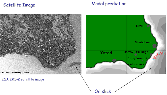
Figure 1. ESA ERS-2 satellite image from June 2nd 2003 at 10 p.m.( same day as the oil spill approaches the Swedish coast, as seen in the lower right corner ) compared by the 3D oil drift model result at the same day and time. Red dots indicate oil at sea surface while light dots indicate oil at subsurface.

On Tuesday morning 3 June 3rd the first oil slicks had stranded on the south coast of Sweden –from Borrby to Sandrishamn. Thursday evening June 5th the wind changed to a strong westerly wind, which caused the oil at the Swedish coastline to drift offshore again. During the night the oil drifted towards Christianø, Frederiksø and Græsholmen – the Danish island group of Ertholmene – located northeast of Bornholm. Friday June 6th oil was still leaking from Fu Shan Hai and was also moving towards the Danish island group of Ertholmene. From early Friday morning three Danish oil-combating vessels were trying to prevent the oil drifting into the coast – by dike and collecting of the oil slick. Saturday June 7th oil polluted the shores and cliffs of Christianø.

3D Oil Drift and Fate Model result

The model predictions were generally in agreement with the oil slick observations described above. The model predicted a severe oil pollution at the Swedish southeast coast – from Borrby in the south up to Simrishamn - 3-4 days after the accident - in agreement with observations. The model predicted an oil pollution of the Swedish coastline to take place 3 June (4 days after the accident) after which the model predicted the oil along the Swedish coastline to drift offshore again and eastwards towards the Danish island group of Ertholmene. The oil was predicted to drift towards the east and strand on Christiansø on June 5.

On the model oil drift animation below one can follow the model predictions of the different oil weathering processes parameter as a function of time, that to say the percentage of oil evaporation, oil dispersed in the subsurface, water content in the oil, etc. Red colour indicates oil at the surface, blue colour oil at subsurface and black colour oil deposited at either the seafloor or coastlinies.

Simulation series

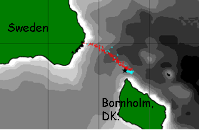
Figure 2. Simulation time: 03.06.03 05:00 UTC. (57 hrs after the oil spill). During the night of 3 June the oil spill polluted the coastline of Sweden from Borrby to Sandrishamn.

Figure 3. Simulation time: 04.06.03 14:00 UTC. (90 hrs after the oil spill) The oil spill has drifted further northwards to Simrishamn and thus polluted a larger part of the Swedish coastline.

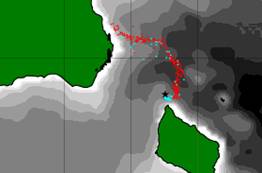
Figure 4. Simulation time: 05.06.03 07:00 UTC. (107 hrs after the oil spill). The oil spill has drifted further northwards.

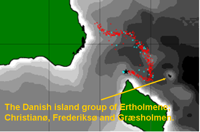
Figure 5. Simulation time: 05.06.03 10:00 UTC. (120 hrs after the oil spill) The oil spill has now drifted offshore towards the Danish island group of Ertholmene –northeast of Bornholm - in agreement with obsrvations.

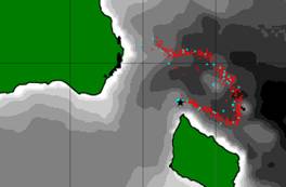
Figure 6. Simulation time: 06.06.03 07:00 UTC. (135 hrs after the oil spill). During the morning of 6 June the oil spill drifted onto the coasts of Ertholmene. In reality the oil first drifted into the island the next morning. However the simulation did not take into account the three oil-combating vessels who early Friday morning were preventing the oil slick to pollute the coastlines.

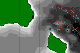
Figure 7. Simulation time: 09.06.03 10:00 UTC. (206 hrs after the oil spill). Oil release and oil slick distribution 8-9 days after the accident. From the release point – at 68-meter depth the simulation indicates an easterly oil drift under the surface – making the oil spill first to become visible at the sea surface a distance from the sunken ship.

The model animations indicate approximately 58% oil floating at the sea surface and approximately 22% oil drifting in the waters below the sea surface.

2D model result

The oil drift was also simulated by use of the MIKE 21-SA 2D oil drift model at DMI. The forecast showed the oil slick to drift northwest and strand on the Swedish south coast of Ystad approximately 25-30 km west of where the oil was observed to strand.

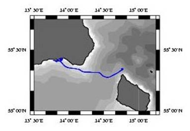
Figure 8. Simulated oil drift by MIKE 21-SA. The plot is a mean track of the oil drift.

The model simulated the released “oil particles” to strand and deposit on the coastline. Particles reaching the coast are considered “stranded” and are not considered in subsequently calculations. The model was therefore not able to simulate that the oil drifted offshore and out on the open sea again and further eastwards and towards the island group of Ertholmene.

The better performance of the 3D-model versus the 2D-model is clearly illustrated by this demonstration case. This is primarily because of the 3D-models ability to simulate the below-surface movements and weathering processes.

Conclusion

In the Fu Shan Hai case, the 3D oil drift and fate model predicted very precisely the oil pollution at the coast of Borrby. The model also predicted the later drift of oil from the Swedish coast zone out on the open sea and towards the sensitive Danish island group of Ertholmene. The Fu Shan Hai forecast is an example of the advances of a 3D oil drift model, that takes into account oil spilled below the surface or at the seabed and calculates the oil spreading and movement at both the subsurface water layers and sea surface.  

Reference

Christiansen, B. M., 2003: 3D Oil Drift and Fate Forecast at DMI. Technical Report No. 03-36. Danish Meteorological Institute, Denmark.